Introduction to GeoSpatial streaming with Apache Spark and Apache Sedona

We are  producing more and more geospatial data these days. Many companies struggle to analyze and process such data, and a lot of this data comes from IOT devices, autonomous cars, applications, satellite/drone images and similar sources. As we can see, there is a need to process the data in a near real-time manner. There are key challenges in doing this, for example how to use geospatial techniques such as indexing and spatial partitioning in the case of streaming data. How can we reduce the query complexity to avoid cross join and make our code run smoothly? How can we apply geohashes and other hierarchical data structures to improve query performance?

Moreover, we need to somehow reduce the number of lines of code we write to solve typical geospatial problems such as objects containing, intersecting, touching or transforming to other geospatial coordinate reference systems.

Apache Spark is one of the tools in the big data world whose effectiveness has been proven time and time again in problem solving.  A lack of native geospatial support can be fixed by adding Apache Sedona extensions to Apache Spark.

Now we can: 

• manipulate geospatial data using spatial functions such as ST_Area, ST_Length etc.
• validate geospatial data based on predicates
• enrich geospatial data using spatial join techniques (stream to table join or stream to stream join).

Let’s try to use Apache Sedona and Apache Spark to solve real time streaming geospatial problems. First we need to add the functionalities provided by Apache Sedona.

How to extend Spark structured streaming applications with geospatial capabilities. 

You can achieve this by simply adding Apache Sedona to your dependencies. 

Scala/Java

Please refer to the project example project 

Python

pip install apache-sedona

You also need to add additional jar files to the spark/jars folder or write them while defining the spark session. You can find an example of how to do this by clicking on this link.

A Spark Session definition should look likes this:

spark = SparkSession. \
    builder. \
    appName('appName'). \
    config("spark.serializer", KryoSerializer.getName). \
    config("spark.kryo.registrator", SedonaKryoRegistrator.getName). \
    config('spark.jars.packages',
         'org.apache.sedona:sedona-python-adapter-3.0_2.12:1.1.0-incubating,org.datasyslab:geotools-wrapper:1.1.0-25.2'). \
    getOrCreate()

After defining the spark session for a scala/java or python application, to add additional functions, serialization geospatial objects and spatial indexes please use the function call as below:

Python

SedonaRegistrator.registerAll(spark)

Scala/Java

SedonaSQLRegistrator.registerAll(spark)

Now that we have all that set up, let's solve some real world problems.

Spatial SQL functions to enrich your streaming workloads

At the moment, Sedona implements over 70 SQL functions which can enrich your data including:

• Geospatial Data Transformations functions such as ST_SubDivide, St_Length, ST_Area, ST_Buffer, ST_isValid, ST_GeoHash etc.
• Geospatial Data predicates such as ST_Contains, ST_Intersects, ST_Within, ST_Equals, ST_Crosses, ST_Touches, ST_Overlaps
• Geospatial Data aggregation ST_Envelope_Aggr, ST_Union_Aggr, ST_Intersection_Aggr
• Constructor functions such as ST_Point, ST_GeomFromText, ST_GeomFromWkb

We can go forward and use them in action.

Filtering Geospatial data objects based on specific predicates

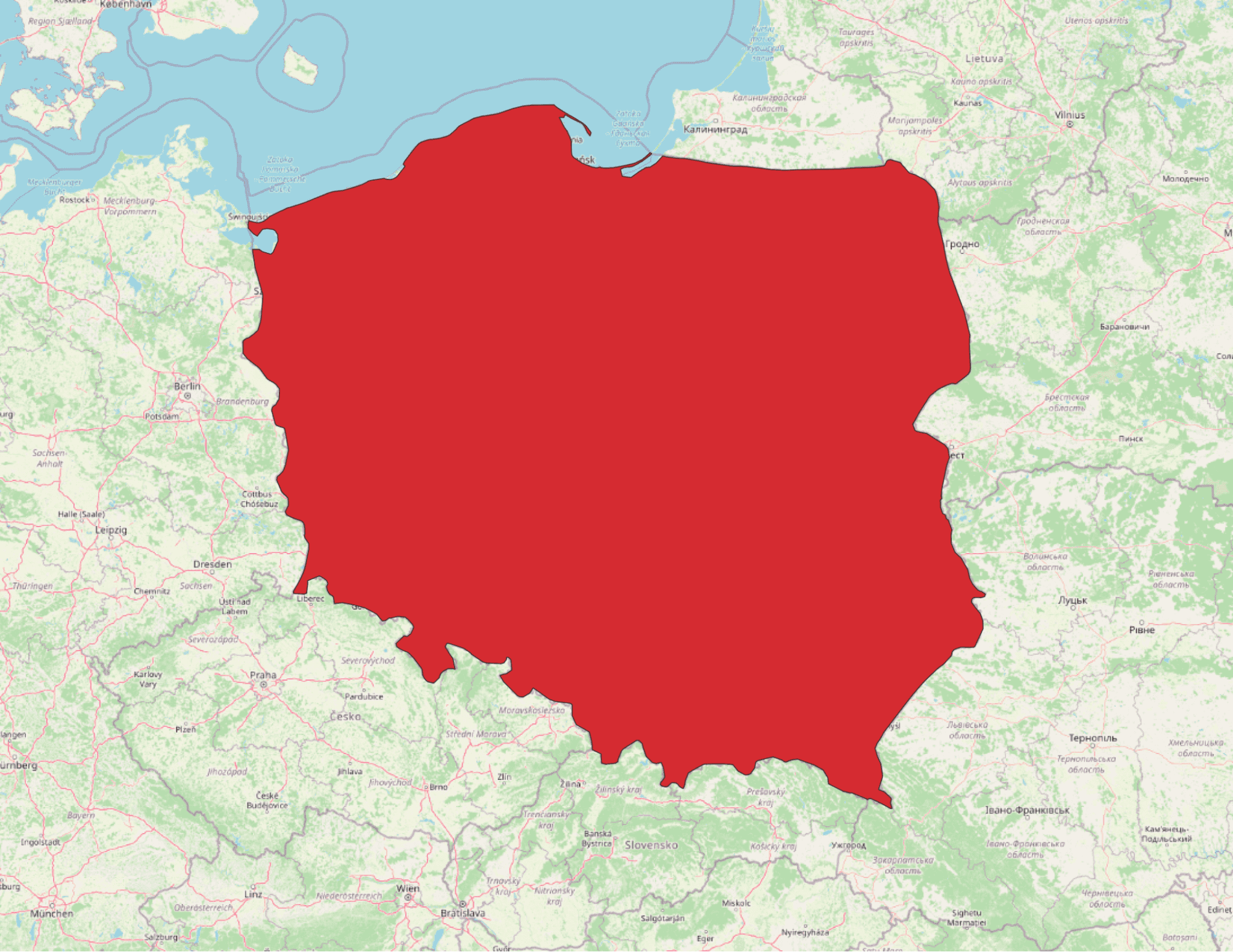
Let's use Poland as an example. 

First of all, we need to get the shape of Poland which  can be achieved by loading the geospatial data using Apache Sedona. You  can download the shapes for all countries here.

For simplicity, let’s assume that the messages sent on kafka topic are in json format with the fields specified below: 

{
  "location": {
    "lon": "21.00",
"lat": "52.00",
"crs": "EPSG:4326"
},
	“velocity”: {
		“value”: 21.0,
		“unitOfMeasure”: “km/h”
	}
	“id”: “11aa7c89-6209-4c4b-bc01-ac22219d6b64”
}

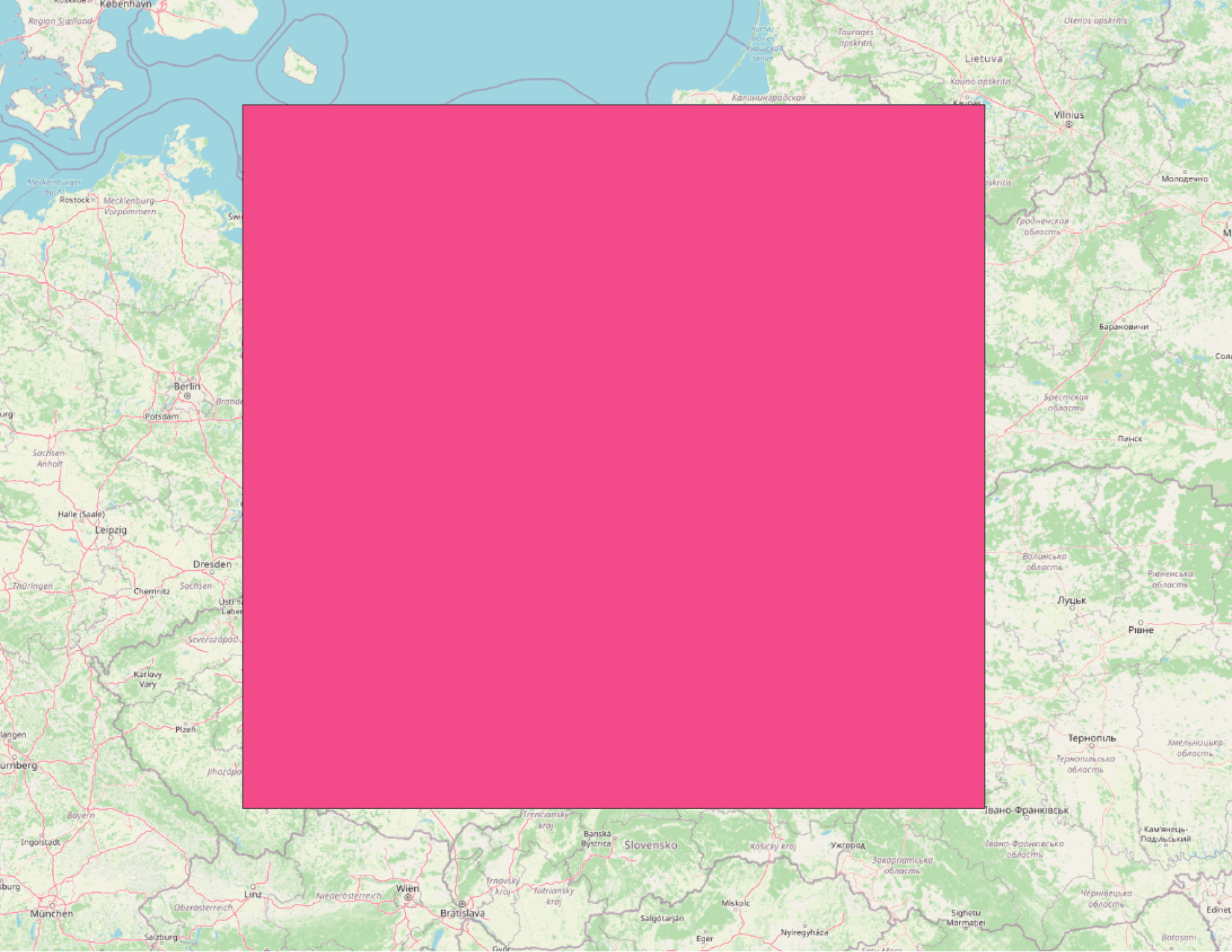
To speed up filtering, first we can reduce the complexity of the query.  For points which lie far away, we can first try to check if it is within the Poland boundary box. If we can, then we should check with more complex geometry.

Creating the geometry of Poland: 

 val countryShapes = ShapefileReader.readToGeometryRDD(
    spark.sparkContext, “location”
  )

 val polandGeometry = Adapter.toDf(countryShapes, spark)
    .filter("cntry_name == 'Poland'")
    .selectExpr("ST_ASText(geometry)", "ST_ASText(ST_Envelope(geometry))")
    .as[(String, String)]
    .collect().head

 val polandShape = polandGeometry._1
 val polandEnvelope = polandGeometry._2

Transformation and filtering step

df
    .selectExpr("decode(value, 'UTF-8') AS json_data", "timestamp")
    .select(from_json($"json_data", schema).alias("measure"), $"timestamp")
    .select(
      expr("ST_Point(measure.location.lon, measure.location.lat)").alias("geom"),
      col("measure"))
    .select(
      expr("""ST_Transform(geom, measure.location.crs, 'epsg:4326')""").alias("geom"),
      col("measure"))
    .filter(
      expr(s"ST_Within(geom, ST_GeomFromWkt('$polandEnvelope'))")
    )
    .filter(
      expr(s"ST_Within(geom, ST_GeomFromWkt('$polandShape'))")
    )

We can easily filter out points which are far away from the Polish boundary box.

Broadcast join for feature enrichment

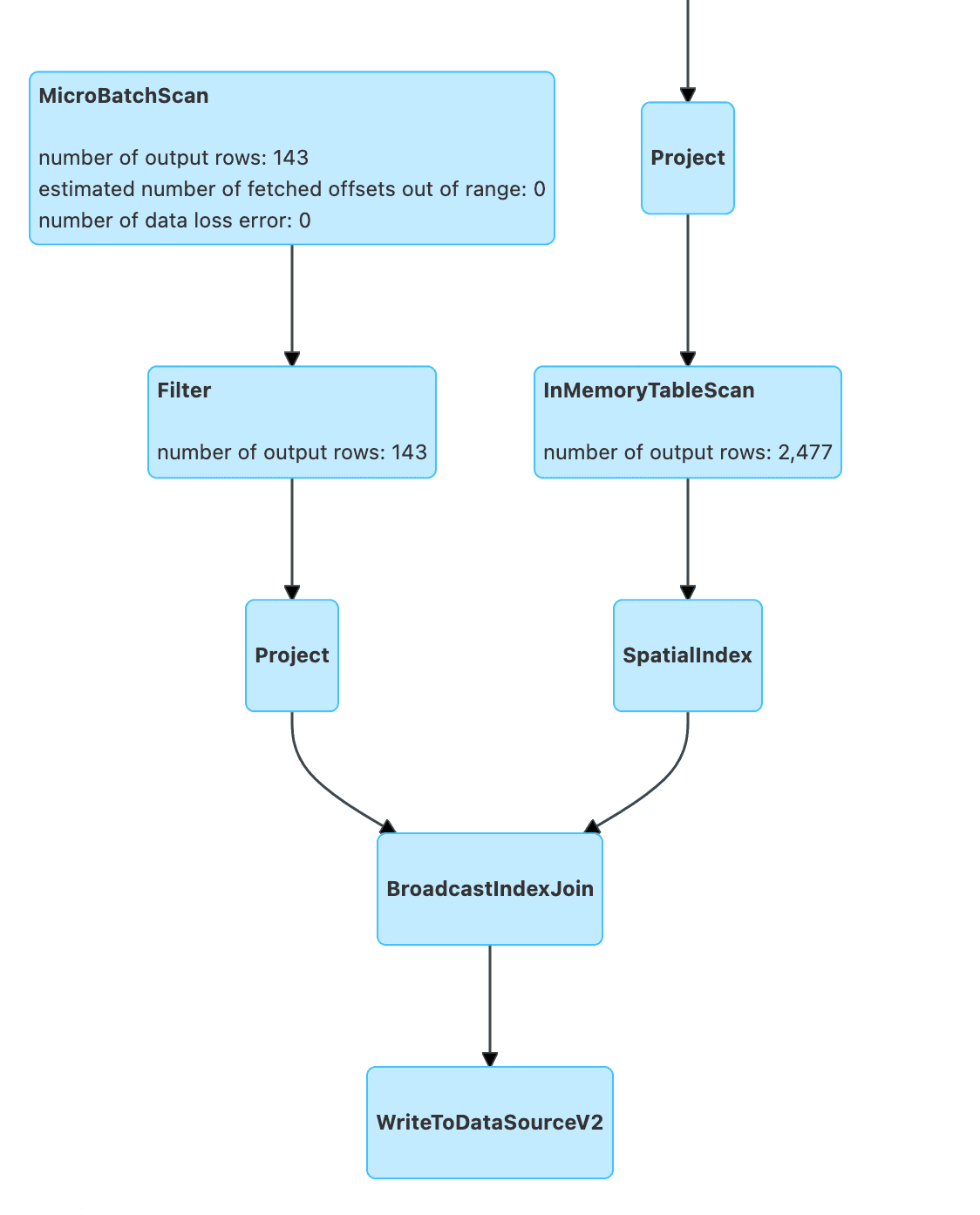
For many business cases, there is the need to enrich streaming data with other attributes. With the use of Apache Sedona, we can apply them using spatial operations such as spatial joins.

Let's stick with the previous example and assign a Polish municipality identifier called  TERYT. To do this,  we need geospatial shapes which we can download from the website. 

First we need to load the geospatial municipalities objects shapes

val municipalities = ShapefileReader.readToGeometryRDD(
    spark.sparkContext,
    "path"
  )

# Transformation to get coordinates in appropriate order and transform them to desired coordinate reference system

 val municipalitiesDf = Adapter.toDf(municipalities, spark)
    .selectExpr("geometry", "JPT_KOD_JE AS teryt")
    .selectExpr("ST_FlipCoordinates(ST_Transform(geometry, 'epsg:2180', 'epsg:4326')) AS geometry", "teryt")
    .cache()

# lets broadcast our data

val broadcastedDfMuni = broadcast(municipalitiesDf)

The next step is to join the streaming dataset to the broadcasted one. A little piece of code has to be added to the previous example (look at Filtering Geospatial data objects based on specific predicates). 

join(broadcastedDfMuni, expr("ST_Intersects(geom, geometry)"))

GeoHash

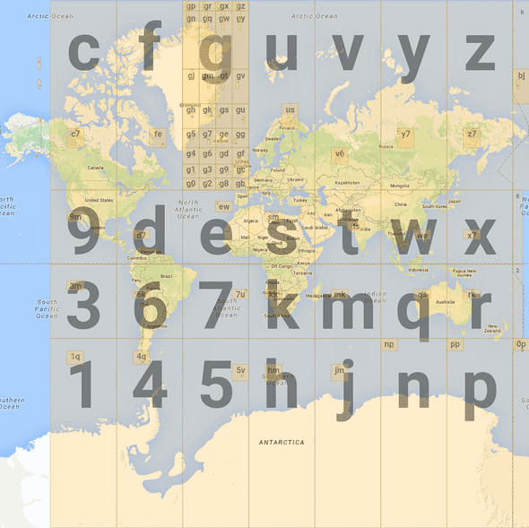
To reduce query complexity and parallelize computation, we need to somehow split geospatial  data into similar chunks which can be processed in parallel fashion. To do this we can use the GeoHash algorithm.

GeoHash is a hierarchical based methodology to subdivide the earth surface into rectangles, each rectangle having string assigned based on letters and digits. Identifier length is based on subdivision level. Example:

lat 52.0004 lon 20.9997 with precision 7 results in geohash u3nzvf7 and as you may be able to guess, to get a 6 precision create a substring with 6 chars which results in u3nzvf.

Indexed Join two data streams

At the moment, Sedona does not have optimized spatial joins between two streams, but we can use some techniques to speed up our streaming job. In our example, we can use municipality identifiers to first match them and then run some geospatial predicates.

leftGeometries
    .join(rightGeometries.alias("right"),
      expr("right_muni_id == left_muni_id")
    )
    .filter("ST_Intersects(left_geom, ST_Buffer(right_geom, 1000))")

Secondly we can use built-in geospatial functions provided by Apache Sedona such as geohash to first join based on the geohash string and next filter the data to specific predicates. 

Example:

for buffer 1000 around point lon 21 and lat 52 geohashes on 6 precision level are:

• 't5q0eq',
• 't5q0er',
• 't5q0et',
• 't5q0ev',
• 't5q0ew',
• 't5q0ex',
• 't5q0ey',
• 't5q0ez',
• 't5q0g2',
• 't5q0g3',
• 't5q0g8',
• 't5q0g9',
• 't5q0gb',
• 't5q0gc',
• 't5q0gd',
• 't5q0gf'.

To find points within the given radius, we can generate geohashes for buffers and geohash for points (use the geohash functions provided by Apache Sedona). Join the data based on geohash, then filter based on ST_Intersects predicate.

Why use Apache Sedona to process streaming data with Apache Spark? 

Apache Sedona provides you with a lot of spatial functions out of the box, indexes and serialization. Therefore, you don’t need to implement them yourself. There are a lot of things going on regarding stream processing. 

Apache Sedona (incubating) is a Geospatial Data Processing system to process huge amounts of data across many machines. At the moment of writing, it supports API for  Scala, Java, Python, R and SQL languages. It allows the processing of geospatial workloads using Apache Spark and more recently, Apache Flink. It's gaining a lot of popularity (at the moment of writing it has 440k monthly downloads on PyPI) and this year should become a  top level Apache project. If you would like to know more about Apache Sedona, check our previous blog “Introduction to Apache Sedona”.

—

Did you like this blog post? Check out our other blogs and sign up for our newsletter to stay up to date!