Deploying efficient Kedro pipelines on GCP Composer / Airflow with node grouping & MLflow
Airflow is a commonly used orchestrator that helps you schedule, run and monitor all kinds of workflows. Thanks to Python, it offers lots of freedom…
Read moreApache Sedona is a distributed system which gives you the possibility to load, process, transform and analyze huge amounts of geospatial data across different machines. It extends Apache Spark with out of the box resilient distributed datasets SRDDs and also brings Spatial SQL to simplify tough problems.
Apache Sedona provides API in languages such as Java, Scala, Python and R and also SQL, to express complex problems with simple lines of code.
For example, you want to find shops within a given distance to the road you can simply write:
SELECT s.shop_id, r.road_id
FROM shops AS s, roads AS r
WHERE ST_Distance(s.geom, r.geom) < 500;
As easy as that, a complex problem is simplified into 3 lines of code. This query gives you all the Sedona optimizations such as:
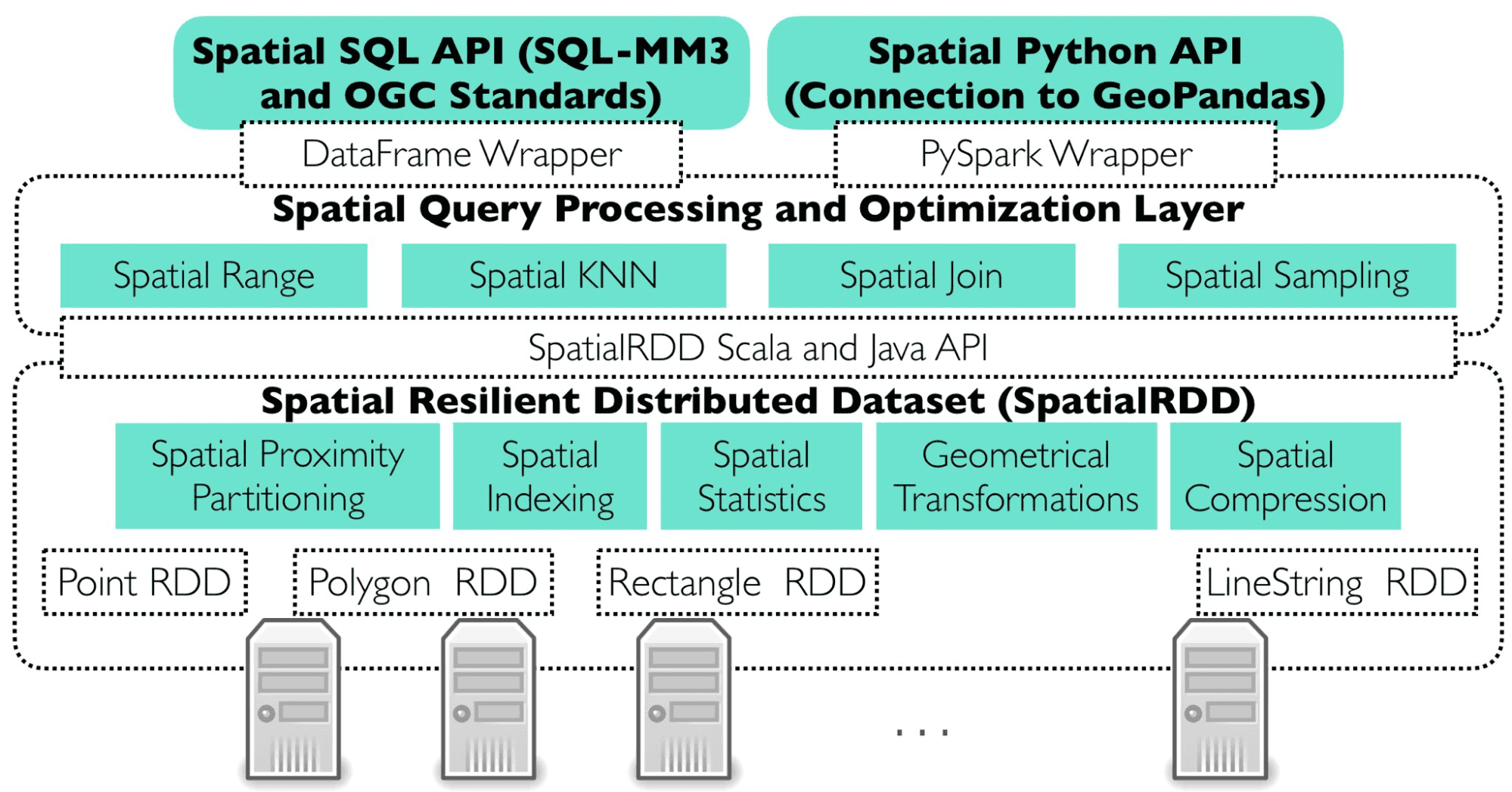
Apache Sedona adds new join plans to Apache Spark to efficiently process data and solve typical spatial problems in a distributed manner. Sedona automatically performs range, join, query and distance join queries. In the case of broadcast joins, it has to be turned on by the user using the broadcast function on a spatially joined dataframe.
This optimization is used when such operations such as ST_Contains, ST_Intersects, ST_Within are utilised when executing the spark join method. The physical plan of the query looks like this:

Optimization is used when finding objects within a given radius. The physical plan looks similar to this:

Useful when data on the right side of the join is small enough to copy on all the machines. Data shuffle and spatial partitioning on the right side can be skipped. By default it is not turned on, it has to be used with the broadcast functions available from the spark.sql.functions. The physical plan looks like this:

Before the spatial join, range filtering is required. Sedona first filters the area then spatially joins dataframes.

To distribute data across machines, Apache Sedona assigns each geometry partition to which it should be processed.


As you can see in the examples, the more points within the area, the smaller the size of the partition (spatial size, width and height).
Currently, Apache Sedona supports two types of spatial partitioning
Apache Sedona creates two indexes while processing huge amounts of geospatial data, globally and locally.
The main goal of the global index is to prune partitions which have no data which will no longer be useful during the query. This in turn speeds up the query due to the fact that there are no workers with empty partitions to process.
Local indexes are created in each partition separately to decrease the number of comparisons between geometries. This is important especially when analyzed geometries are complex such as polygons with huge amounts of vertices. Currently, Apache Sedona supports three types of indexes:
This is useful when data on one side of a spatial join is small enough to spread copies of the data across the machines. This can significantly reduce the amount of resources and processing time; there is no need to spatially partition one side of the join so we can omit costly shuffles.
To decrease the impact of processing geospatial data, Apache Sedona implements object serialization. The methodology is definitely faster than the default implemented in Spark, kryo serializer. Serializing Spatial objects such as points, polygons and linestrings is not enough - in many cases spatial index can be as large as, or even greater in size than spatial objects overall. Apache Sedona also serializes these objects to reduce the memory footprint and make computations less costly.
To serialize the Spatial Index, Apache Sedona uses the DFS (Depth For Search) algorithm.
Apache Sedona uses wkb as the methodology to write down geometries as arrays of bytes. An example of decoding geometries looks like this:
POINT(21 52)
Example Point(50.323281, 19.029889)
1 | 1 0 0 0 |-121 53 -107 69 97 41 73 64 | -103 -126 53 -50 -90 7 51 64
Where the first byte is byte order, the next four correspond to the geometry data type and the last 16 encode X and Y coordinates accordingly.
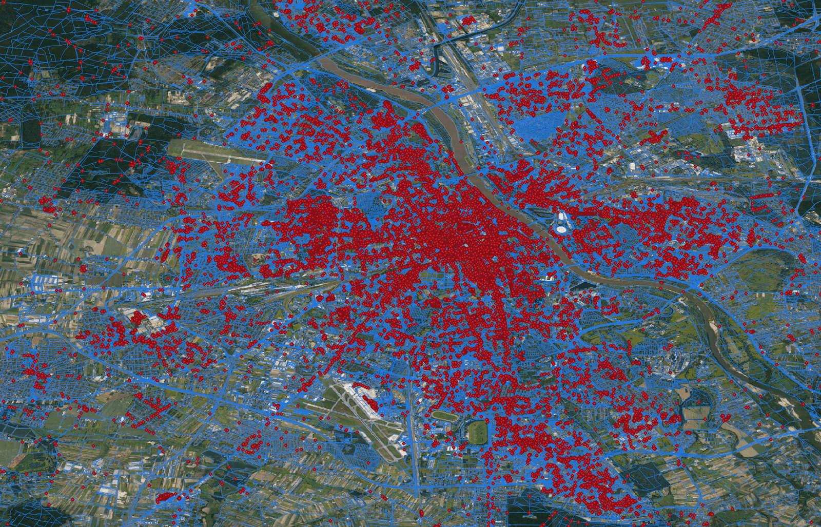
In this example, we will try to find restaurants within a 200m radius from certain roads in the Masovian voivodeship. First we write the query using SQL API, after that we switch to core RDD API where defined spatial partitioning and spatial indexing can be chosen.
SQL API
Let's assume that our dataset looks like this:
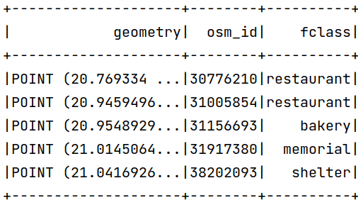
The dataset with roads already loaded to geospatial dataframe:
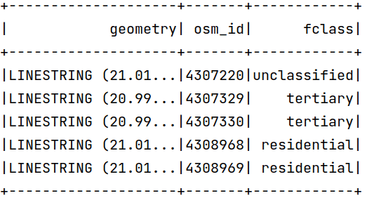
As you can see, dataframes have coordinates in degrees but the predicate is in meters - Apache Sedona does not transform coordinates automatically to meters. To change the coordinates to meters we can use the ST_Transform function. The coordinates in EPSG:2180 should look like this:
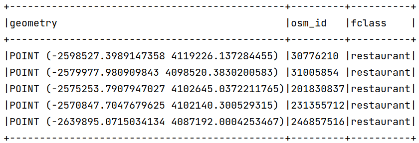
To express the solution using Scala and SQL API, we can write a simple code:
val restaurants = sparkSession.read.parquet("pois").where("fclass == 'restaurant'")
 .withColumn("geometry", expr("ST_Transform(geometry, 'EPSG:4326', 'EPSG:2180')"))

val roads = sparkSession.read.parquet("roads")
 .withColumn("geometry", expr("ST_Transform(geometry, 'EPSG:4326', 'EPSG:2180')"))

restaurants.createOrReplaceTempView("restaurants")

roads.createOrReplaceTempView("roads")

sparkSession.sql(
 """
   |SELECT rt.osm_id AS rt_id, rd.osm_id AS rd_id, ST_Distance(rd.geometry, rt.geometry) AS dist
   |FROM roads AS rd, restaurants AS rt
   |WHERE ST_Distance(rt.geometry, rd.geometry) <= 200
   |""".stripMargin
)
Which creates a physical plan:

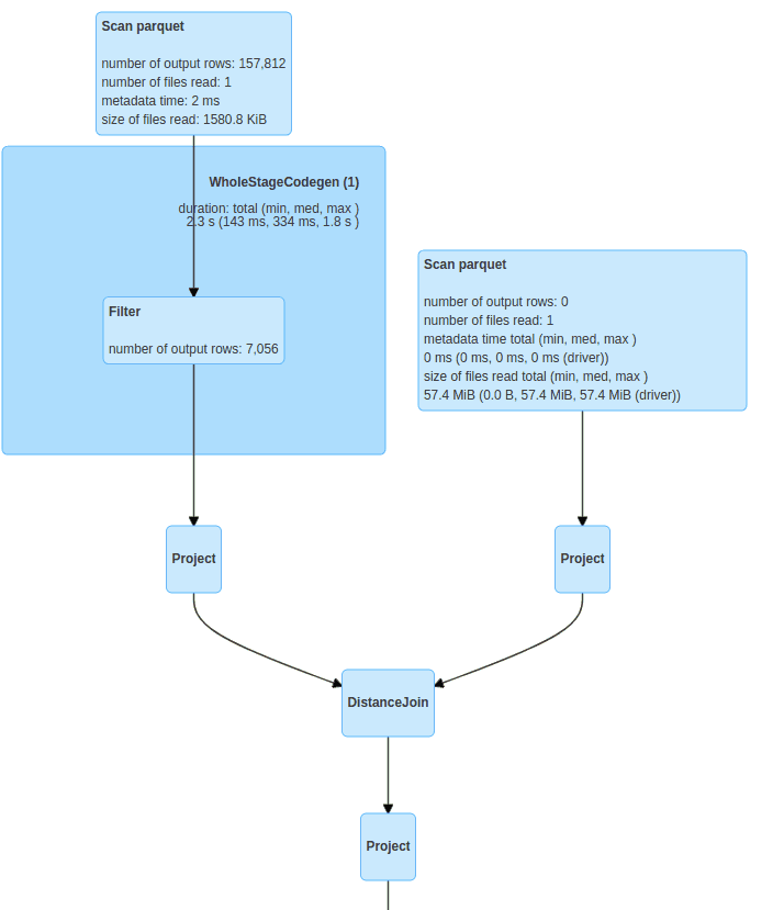
Due to spark limitations, the Apache Sedona RDD API is faster than the DataFrame API, the equivalent code used previously looked like this:
// finding desired transformation
val sourceCrsCode = CRS.decode("EPSG:4326")
val targetCrsCode = CRS.decode("EPSG:2180")
val transformation = CRS.findMathTransform(sourceCrsCode, targetCrsCode, false)

// reading shapefile format to SpatialRDD
val pois = ShapefileReader.readToGeometryRDD(
 sparkSession.sparkContext, "pois"
)

// filter to restaurants and transform to metric coordinate system
pois.rawSpatialRDD = pois.rawSpatialRDD.filter(row => row.getUserData.toString.split("\t")(2) == "restaurant")
pois.rawSpatialRDD = pois.rawSpatialRDD.repartition(100)
pois.rawSpatialRDD = pois.rawSpatialRDD.map(geom => JTS.transform(geom, transformation))

// reading roads to SpatialRDD
val roads = ShapefileReader.readToGeometryRDD(
 sparkSession.sparkContext, "roads")

// transforming to metric coordinate system
roads.rawSpatialRDD = roads.rawSpatialRDD.map(geom => JTS.transform(geom, transformation))

// Creating Circle rdd based on points and given radius
val circleRDD = new CircleRDD(roads, 200)

// analyzing data to optimize spatial partitioning
circleRDD.analyze()

// apply spatial partitioning
circleRDD.spatialPartitioning(GridType.KDBTREE)

// building spatial index, we also apply spatial indexing on spatial partitions to prune empty partitions
circleRDD.buildIndex(IndexType.RTREE, true)

// apply spatial partitioning from left side of the join to the right side
pois.spatialPartitioning(circleRDD.getPartitioner)

// performing spatial join between roads buffers and restaurants, as third argument we chose to use index and as
// fourth we still match points which lays on boundaries.
val spatialResult = JoinQuery.DistanceJoinQueryFlat(pois, circleRDD, true, true)

// converting result to dataframeApache Sedona provides the possibility of loading the data from various data sources such as:
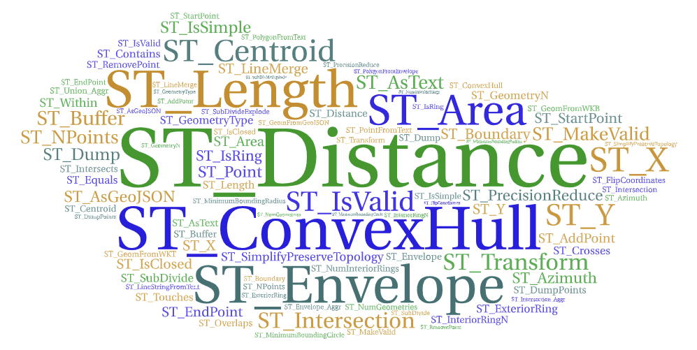
Express complex problems with a simple SQL query:
SELECT superhero.name
FROM city, superhero
WHERE ST_Contains(city.geom, superhero.geom)AND city.name = 'Gotham'
Load the data using geopandas, the list of shapely objects, convert the sequence of locationtech geometry objects directly into the Geospatial Data Frame.
Install via PyPI, add additional jars to the spark session and that’s all. In the case of jvm based applications, add Apache Sedona as a dependency and create a fat jar.
You can scale your geospatial workflows across many machines.
Run it everywhere
Apache Sedona (incubating) is promising library which gives the possibility to scale geospatial data processing workloads, it can be easily deployed on the cloud such as AWS, Azure, GCP. It provides APIs in most popular languages like Java, Scala, Python, R.
Apache Sedona major properties:
Usability: Comprehensive geospatial data wrangling and transformation API
Scalability: Sedona can perform a spatial join on 4 billion of points data and 200 thousand polygon data in ~3 minutes on 4 machines
Integrability: integration with modern data science infrastructure and GIS tools
Deployability: Easy deployment on major cloud providers
Popularity: ~1k stars on GitHub and almost 200k monthly downloads on PyPI
If you want to know more, feel free to check the Apache Sedona documentation.
Did you like this blog post? Check out our other blogs and sign up for our newsletter to stay up to date!
Airflow is a commonly used orchestrator that helps you schedule, run and monitor all kinds of workflows. Thanks to Python, it offers lots of freedom…
Read moreIn today's fast-paced business environment, companies are increasingly turning to real-time data to gain a competitive edge. One of the examples are…
Read moreAcquiring unlabeled data is inherent to many machine learning applications. There are cases when we do not know the result of the action provided by…
Read moreIn today's world, real-time data processing is essential for businesses that want to remain competitive and responsive. The ability to obtain results…
Read moreWhat are Large Language Models (LLMs)? You want to build a private LLM-based assistant to generate the financial report summary. Although Large…
Read moreBusinesses across industries are using advanced data analytics and machine learning to revolutionize how they operate. From detecting anomalies to…
Read moreTogether, we will select the best Big Data solutions for your organization and build a project that will have a real impact on your organization.
What did you find most impressive about GetInData?